
Click here to see other posts about XRD
The fee of the quantitative Rietveld analysis using MAUD software depends on the XRD pattern complexity
Payment Upon Completion
 Send your patterns...
1. Introduction
Today several instruments for fast spectra recording are available. In most cases the difficulty
is to process and analyze the data quickly in a reliable way. The Maud program, in one of its
many undocumented features, can be used to process a list of analyses in batch mode from the
console without requiring the interface. This is useful to process quickly similar spectra or launch
a slow/time consuming refinement in a remote computer without recurring to the interface that
would need to open a session involving the remote display setting.

The overall procedure is to prepare the analysis locally using the interface or to prepare a starting point for a series of spectra
(one common starting point) also using the interface, then to prepare an instruction file in CIF like
format to specify the analyses, the spectra and the kind of refinement to conduct and finally to run
Maud in batch mode providing the instruction file previously prepared. The program will run and
process one analysis at time and prepare an output file extracting some key information (either the
default or some to be specified) in a format suitable to be imported in spreadsheet or graphical
programs to analyze the results.
As an example we will show the procedure to analyze a series of ball milled Cu-Fe mixed powders
in which two different phases may form with a different composition. By an automatic Rietveld
analysis performed in batch mode we will extract information about phase content [2, 1], crystallite
and microstrain for each sample/spectrum. The analysis is further complicated from the fact that
the powders milled at higher energy show the presence of planar defects [5] and texture arising
from sample preparation and the platelet like shape of the grains [3].
2 Analysis and procedure
In this section we will present the procedure to analyze 25 spectra of Cu-Fe different samples. The
spectra has been collected by a Philips X-pert system in Le Mans at the LPEC laboratory of the
1
University du Maine, thanks to A. Gibaud.
2.1 Analysis preparation through the interface
We start the Maud program and load all the datafiles together to check their integrity and to prepare
a common starting analysis file. A plot of all spectra and their differences is available in Figure 1.
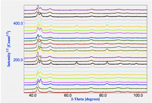
presence of both fcc and bcc phases, but not in all.
We load the two possible phases, bcc iron and fcc copper, from the Maud database. By computing
the spectra once and comparing them visually with the experimental spectra we may notice that
for some samples, milled at longer time, an alloyed fcc phase form (out of equilibrium) and the
bcc iron disappears. Unluckily we could not use the copper rich phase cell parameter to monitor
the Fe content in it as the cell parameter tends to growth as a result probably of oxygen entrapping.
In a first attempt we discovered the spectra were affected by texture, anisotropic crystallite sizes
and microstrain as well as planar defects (especially on the Cu like phase). So we decide here
to include also texture and anisotropic/planar defects effects in the analysis. For both the bcc
and fcc phases we select in the proper panel the Popa model for anisotropic broadening [4], the
Warren model for planar defects and the harmonic model for texture (specifying cylindrical sample
symmetry and Lmax = 6 in the options; it is required by the experiment geometry).
Next step was to adjust the cell parameters for both bcc and fcc phases in order to get a mean
starting value good for all spectra (especially for the fcc); and to adjust the crystallite value to a
good starting point (around 200 angstrom) obtaining peak shapes a little sharper than in the less
broadened spectrum. The background constant parameter was also adjusted to the value of the
spectrum with the lower background. Actually only the cell parameter adjustment is critical, the
background one is even not necessary.
Finally we remove all the spectra (we will specify which datafile to use for each analysis later in an
instruction file) and save the analysis containing everything except the spectrum/a. For the purpose
of this article we save the analysis with the name: FeCustart.par.
2.2 Preparation of the instruction file and batch processing
To run Maud in batch we need to write an instruction file containing the list of analyses to execute
one at time. The file is in CIF format but containing some terms not available in the official CIF
dictionary, but that Maud recognize. All the analyses to be performed are specified through the
loop CIF instruction. The first term of the loop must be the one specifying the starting analysis
file to be loaded (full path in unix convention) and then the others to instruct Maud for the kind
of analysis to perform, iterations and eventually datafile to load and name of the file were to save
the analysis. Additional keywords can be used to append specific results to a file for spreadsheet
analysis. The simplest instruction file is something containing the following:
First example (paths for windows):
loop
riet analysis file
riet analysis iteration number
2
´//C:/mypathfortheanalysis/analysis1.par´ 5
´//C:/mypathfortheanalysis/analysis2.par´ 3
´//C:/mypathfortheanalysis/analysis3.par´ 7
The analysis1.par (or 2 or 3) are some analyses files prepared with Maud, containing also
the datafile/spectrum, already set for the parameters to be refined and saved just ready for the refinement step. Maud will load each analysis, starts the refinement with the number of iterations
specified and save the analysis with the refined parameters under the same name. The analyses can
be loaded at end in Maud (with the interface) to see the result of the refinement.
In the case of the Cu-Fe we need to perform some more steps: first we start from one common analysis point (the FeCustart.par analysis file) but we want to specify different datafiles; second
we want to perform a full automatic analysis in which Maud performs different cycles deciding
which parameters to refine at each step and third we will specify the name of each analysis for the
saving process and a file name were to append some selected results in a tab/column format for
subsequent easy loading in a spreadsheet program.
Cu-Fe example:
loop
riet analysis file
riet analysis iteration number
riet analysis wizard index
riet analysis fileToSave
riet meas datafile name
riet append simple result to
´//mypath/FeCustart.par´ 7 13 ´//mypath/FECU1010.par´ ´//mypath/FECU1010.UDF´
´//mypath/FECUresults.txt´
´//mypath/FeCustart.par´ 7 13 ´//mypath/FECU1011.par´ ´//mypath/FECU1011.UDF´
´//mypath/FECUresults.txt´
…………(lines with all the other 23 datafiles omitted for brevity)
´//mypath/FeCustart.par´ 7 13 ´//mypath/FECU1038.par´ ´//mypath/FECU1038.UDF´
´//mypath/FECUresults.txt´
With this instruction file (that we save under the name: fecu.ins) we specify for example that
as a first analysis, Maud has to load the FeCustart.par file, then to load in the analysis the
FECU1010.UDF datafile, to perform the automatic analysis number 13 (in the wizard panel of
Maud the automatic analysis number 13 is the texture analysis; we need to refine also the texture
parameters along with phase analysis and microstructure) and to use 7 iterations for each cycle (the
texture automatic analysis is composed by 4 cycles) to ensure sufficient convergence. At the end
the analysis is saved with the name FECU1010.par and simple selected results will be appended
in the file FECUresults.txt. The simple results saved in the spreadsheet like file are some of
the most used parameters and results. It is possible to specify the parameters we want in output
using the CIF word riet append result to (in addition or as an alternative), but in the
preparation of the starting analysis file in the Maud interface, the parameters to be added to the
results must be specified by turning to true the switch in the output column of the parameter list
window or panel.
Now to run Maud in batch in the console (
where the Maud.jar is located the following:
DOS (everything in the same line): java -mx512M -cp
“Maud.jar;lib\miscLib.jar;lib\JSgInfo.jar;lib\jgaec.jar;lib\ij.jar”
it.unitn.ing.rista.MaudText -f fecu.ins
Unix (everything in the same line): java -mx512M -cp
Maud.jar:lib/miscLib.jar:lib/JSgInfo.jar:lib/jgaec.jar:lib/ij.jar
it.unitn.ing.rista.MaudText -f fecu.ins
For Mac OS X, it is advised to use the generic Unix Maud installation (or to change the path to
the jar files). Before to run Maud in batch mode it is important to run Maud interactive (with the
interface) at least once to create and extract the databases, examples and preferences folder.
2.3 Analysis of results
After running Maud in batch mode, we can check quickly the results by loading the results file
FECUresults.txt in a spreadsheet program. The results are arranged in rows and separated
by tabs. The first row contains the column titles, each subsequent row a different analysis. The
Rwp value for each analysis is reported in the second column and the biggest value found was
5.6% as an indication of the success of the analysis. As an example we report in Figure 2 the
graphical correlation of the copper-rich phase percentage and its mean crystallite value as found
in the analysis versus the sample number. The files and examples used in this articles will be
uploaded in a tutorial in the Maud web page along with some additional files with the batch mode
commands for an easier use.

obtained by the automatic batch mode analysis. The plot has been created from the results file
saved by Maud.
3 How to get Maud 2.0 and further informations
For this analysis we need Maud version 2.037 or later and it can be freely downloaded from the
Maud web page at http://www.ing.unitn.it/ maud for the preferred platform. There are two archives
for Windows and Mac OS X plus a generic unix version that can be used for Linux, Solaris or
every unix based system with a Java 2 virtual machine installed. The new version 2.0 has a new
interface focused on reducing the effort of a new user and simplifying the most common tasks.
Some particularity of the new version respect to the previous one are (most of them to provide
some useful routines for ab-initio structure solution):
• Different minimization/search algorithms selectable: Marquardt least squares, Evolutionary
algorithm, Simulated annealing, Metadynamic search algorithm. As an example the evolutionary algorithm can be used in the early steps of the refinement to select the proper starting
solution and the Marquardt to drive it to convergence.
4
• Possibility to use crystallites and microstrain distributions for peak shape description instead
of analytical fixed shape functions.
• Maximum Entropy Electron Map full pattern fitting. An electron map can be used for fitting
instead of atoms.
• Full pattern fitting by a list of peaks. Either an arbitrary list of peaks (each one with its own
position, intensity and shape), or simply a list of structure factors to be imported, instead of
a list of atoms.
• Indexing directly on the pattern, selecting the Le Bail fit and the evolutionary algorithm for
the cell search. This may be used to improve a difficult indexing or a partly done one.
• Introduction of fragments. So fragment search can be done directly on the pattern or on a
list of extracted structure factors.
• Energy minimization. At the moment only the simple repulsion energy is completed. Other
energy principles are under completition.
• Spectra integration from image plate or CCD transmission/reflection 2D images. Center,
tilting errors and distance from sample can be refined in the spectra fitting.
Bugs and errors should be reported to the author through the bug reporter web page; questions in
the Maud forum accessible from the Maud web page.
In a future article we will report the instructions on how to modify/extend the program by little Java programming or provide a new alternative model/plugin for the instrument or the structure/microstructure or datafiles importing.
References
[1] D. L. Bish and S. A. Howard. J. Appl. Cryst., 21, 86–91, 1988.
[2] R. J. Hill and C. J. Howard. J. Appl. Cryst., 20, 467–474, 1987.
[3] L. Lutterotti and S. Gialanella. Acta Mater., 46(1), 101–110, 1998.
[4] N. C. Popa. J. Appl. Cryst., 31, 176–180, 1998.
[5] B. E. Warren. X-ray Diffraction. Addison-Wesley, Reading, MA, 1969
Author: Luca Lutterotti
Dipartimento di Ingegneria dei Materiali e delle Tecnologie Industriali
Universita di Trento, 38050 Trento, Italy `
E-mail: Luca.Lutterotti@ing.unitn.it
WWW: http://www.ing.unitn.it/ maud